Example of MarginalDist Class
This example demonstrates the use of the MarginalDist class to generate synthetic data for a univariate dataset.
Import Libraries
# LOAD DEPENDENCIES
import pprint, sys, os
import matplotlib.pyplot as plt
import numpy as np

# Add path (if necessary)
dir_path = os.path.dirname(os.path.realpath(__file__))
par_dir = os.path.dirname(dir_path)
sys.path.insert(0, par_dir)

from bdarpack.MarginalDist import MarginalDist
from scipy import stats
Build Plot Area
fig, (ax1, ax2) = plt.subplots(1,2)
Generate random data
In this example, we use the scipy stats package to generate a fictitious sample, based on a gamma distribution.
# GENERATE A "FICTIONAL" DATA SAMPLE USING SCIPY
a = 2
loc = 2
scale = 8
samples = stats.gamma.rvs(a=a, loc=loc, scale=scale, size=4000)

# VISUALISE THEORETICAL PDF, CDF AND HISTOGRAM OF GENERATED DATA
# Plot Histogram of Data Sample
ax1.hist(samples, density=True, bins='auto', alpha=0.8, color='blue', label=f'Histogram of Original Samples n={(len(samples))}')

# Plot PDF of Data Sample
x = np.linspace(np.min(samples), np.max(samples), 100)
sample_pdf = stats.gamma.pdf(x=x, a=a, loc=loc, scale=scale)
ax1.plot(x, sample_pdf, 'b-', lw=1, label='Actual PDF using true parameters')

# Plot CDF of Data Sample
x = np.linspace(np.min(samples), np.max(samples), 100)
sample_cdf = stats.gamma.cdf(x=x, a=a, loc=loc, scale=scale)
ax2.plot(x, sample_cdf, 'b-', lw=1, label='Actual CDF using true parameters')
Generate synthetic data
Next, we try to learn the underlying distribution of the generated data. Since the data only has one variable, the MarginalDist class is already sufficient.
# INITIALISE A MARGINALDIST CLASS
univariate = MarginalDist(debug=True)

# LEARN THE OPTIMAL DISTRIBUTION FROM THE DATA SAMPLES
univariate.fit(data=samples)
print(f"optimum univariate: {univariate.fitted_marginal_dist}")

# PLOT THE LEARNED PDF, CDF, AND HISTOGRAM OF SYNTHETIC SAMPLES
# Plot Learned CDF
x = np.linspace(np.min(samples), np.max(samples), 100)
learned_cdf = univariate.cdf_wrapper(data=x)
ax2.plot(x, learned_cdf, 'k-', lw=1, label='Fitted CDF using learned parameters')

# Plot Learned PDF
x = np.linspace(np.min(samples), np.max(samples), 100)
learned_pdf = univariate.pdf_wrapper(data=x)
ax1.plot(x, learned_pdf, 'k-', lw=1, label='Fitted PDF using learned parameters')

# Create a synthetic sample from learned parameters
x = stats.uniform.rvs(size=5000)
learned_ppf = univariate.ppf_wrapper(data=x)
ax1.hist(learned_ppf, density=True, bins='auto', alpha=0.8, color='gray', label=f"Histogram of Synthetic Samples n={len(learned_ppf)}")
Sample Output
Fitting data with known parametric distributions...
Fitting data with beta:: kstat: 0.008172649641283392:: pvalue: 0.9500962142965577
Fitting data with laplace:: kstat: 0.10698355129539623:: pvalue: 2.53940293993326e-40
Fitting data with loglaplace:: kstat: 0.04875553618279055:: pvalue: 1.0570495250612113e-08
Fitting data with gamma:: kstat: 0.0076758003704006095:: pvalue: 0.9710713107419339
Fitting data with gaussian:: kstat: 0.09376866669868594:: pvalue: 4.645675962787757e-31
Fitting data with student_t:: kstat: 0.08774938698900313:: pvalue: 3.0109710266979776e-27
Fitting data with uniform:: kstat: 0.5327760567138355:: pvalue: 0.0
optimum univariate: gamma
Parameters used for generating CDF:/n {'df': 100, 'loc': 1.9389883076225938, 'scale': 8.112381524781696, 'a': 2.0005591824545768, 'b': 1, 'c': 1, 'ecdf': {}, 'gaussian_kde': {}}
Parameters used for generating PDF:/n {'df': 100, 'loc': 1.9389883076225938, 'scale': 8.112381524781696, 'a': 2.0005591824545768, 'b': 1, 'c': 1, 'ecdf': {}, 'gaussian_kde': {}}
Parameters used for generating PPF:/n {'df': 100, 'loc': 1.9389883076225938, 'scale': 8.112381524781696, 'a': 2.0005591824545768, 'b': 1, 'c': 1, 'ecdf': {}, 'gaussian_kde': {}}
PLOT STUFF
ax1.legend(loc='best', frameon=False)
ax2.legend(loc='best', frameon=False)
plt.show()
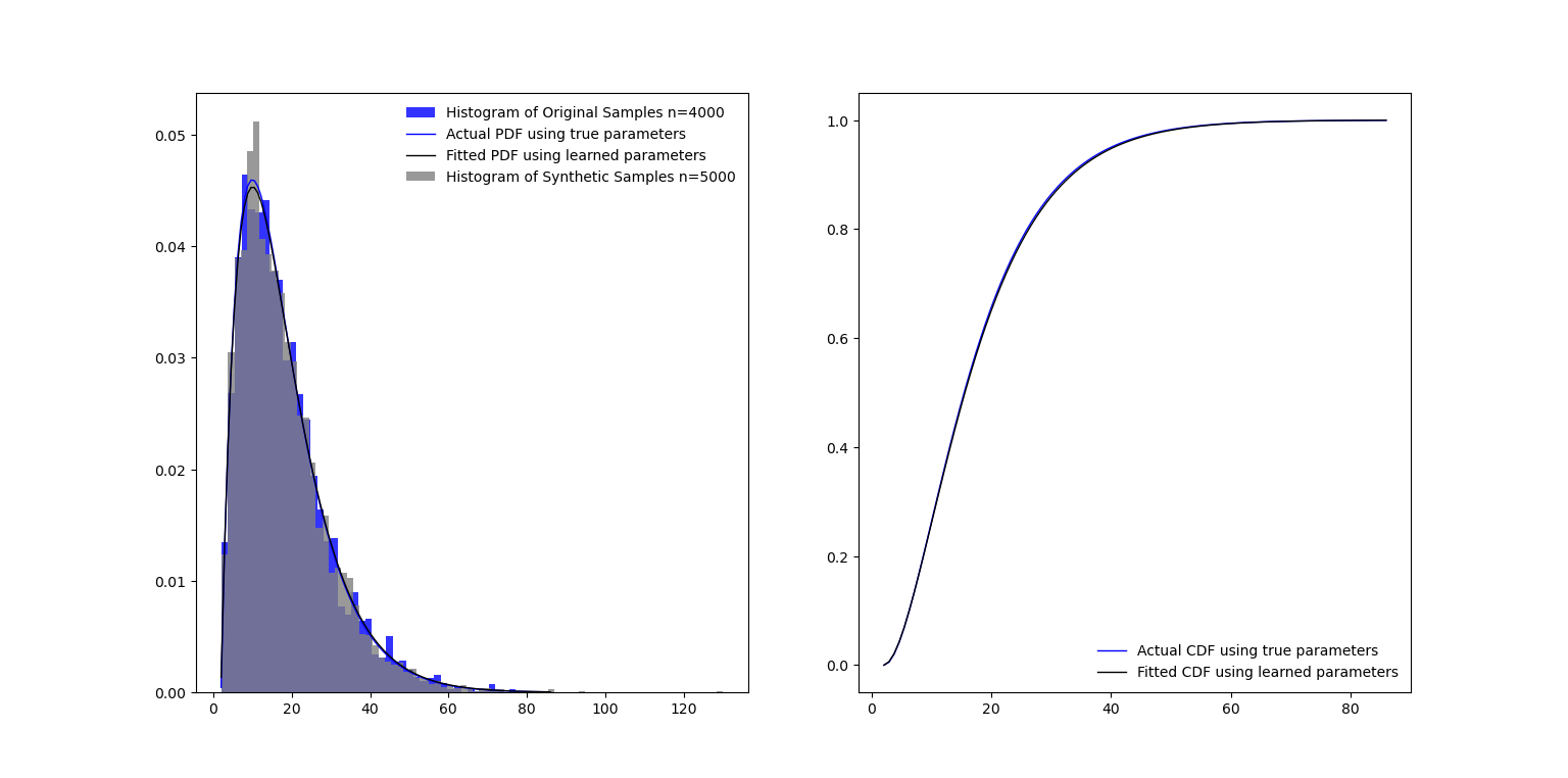
Plot of learned distribution and generated synthetic data samples
Example 2 of MarginalDist Class
In this example, we demonstrate the use of the MarginalDist class to generate synthetic data for a univariate dataset, when the dataset does not follow a known distribution.
Generate random data
In this example, we use the scipy stats package to generate a fictitious sample, based on a mixed gamma and Gaussian distribution.
# GENERATE A "FICTIONAL" DATA SAMPLE USING SCIPY
samples_1 = stats.gamma.rvs(a=4, loc=2, scale=5, size=400)
samples_2 = stats.norm.rvs(loc=60, scale=6, size=400)
samples = np.concatenate((samples_1, samples_2))
Generate synthetic data
Next, we try to learn the underlying distribution of the generated data. Since the data only has one variable, the MarginalDist class is already sufficient.
# INITIALISE A MARGINALDIST CLASS
univariate = MarginalDist(debug=True)

# LEARN THE OPTIMAL DISTRIBUTION FROM THE DATA SAMPLES
univariate.fit(data=samples)
print(f"optimum univariate: {univariate.fitted_marginal_dist}")

# PLOT THE LEARNED PDF, CDF, AND HISTOGRAM OF SYNTHETIC SAMPLES
# Plot Learned CDF
x = np.linspace(np.min(samples), np.max(samples), 100)
learned_cdf = univariate.cdf_wrapper(data=x)
ax2.plot(x, learned_cdf, 'k-', lw=1, label='Fitted CDF using learned parameters')

# Plot Learned PDF
x = np.linspace(np.min(samples), np.max(samples), 100)
learned_pdf = univariate.pdf_wrapper(data=x)
ax1.plot(x, learned_pdf, 'k-', lw=1, label='Fitted PDF using learned parameters')

# Create a synthetic sample from learned parameters
x = stats.uniform.rvs(size=5000)
learned_ppf = univariate.ppf_wrapper(data=x)
ax1.hist(learned_ppf, density=True, bins='auto', alpha=0.8, color='gray', label=f"Histogram of Synthetic Samples n={len(learned_ppf)}")
Sample Output
Fitting data with known parametric distributions...
Fitting data with beta:: kstat: 0.15218241984053915:: pvalue: 1.2146709184078006e-16
Fitting data with laplace:: kstat: 0.2016538619963058:: pvalue: 5.400890340048729e-29
Fitting data with loglaplace:: kstat: 0.23085243173668069:: pvalue: 5.761247455714581e-38
Fitting data with gamma:: kstat: 0.1739346795510226:: pvalue: 1.231265354302602e-21
Fitting data with gaussian:: kstat: 0.1706894482350294:: pvalue: 7.563699611893537e-21
Fitting data with student_t:: kstat: 0.17066442930791947:: pvalue: 7.669253557944495e-21
Fitting data with uniform:: kstat: 0.10784867680944032:: pvalue: 1.4745236262854905e-08
No good distributions found, using non-parametric estimation...
Fitting data with gaussian_kde:: kstat: 0.043047521739585815:: pvalue: 0.10015583588080923
optimum univariate: gaussian_kde
Parameters used for generating PDF:/n {'df': 100, 'loc': 0, 'scale': 0.2626527804403767, 'a': 1, 'b': 1, 'c': 1, 'ecdf': {}, 'gaussian_kde': {'x': array([-101.39095449, -101.38095449, -101.37095449, ...,  184.51904551,
        184.52904551,  184.53904551]), 'u': array([2.51191352e-85, 5.11203884e-85, 7.80346492e-85, ...,
       1.00000000e+00, 1.00000000e+00, 1.00000000e+00])}}
PLOT STUFF
ax1.legend(loc='best', frameon=False)
ax2.legend(loc='best', frameon=False)
plt.show()
Plot of learned distribution and generated synthetic data samples
